Deep Learning for Astronomical Image Processing
InTheArt Seminar, Nov. 20th 2020
François Lanusse


slides at eiffl.github.io/talks/ITA2020
the Rubin Observatory Legacy Survey of Space and Time
- 1000 images each night, 15 TB/night for 10 years
- 18,000 square degrees, observed once every few days
- Tens of billions of objects, each one observed $\sim1000$ times
Previous generation survey: SDSS
Image credit: Peter Melchior
Current generation survey: DES
Image credit: Peter Melchior
LSST precursor survey: HSC
Image credit: Peter Melchior
Outline of this talk
Where can Deep Learning help address the challenges of modern surveys ?
- Low level image processing
- Solving Inverse Problems
- Probabilistic inference
Deep detection of gravitational lenses
Work in collaboration with:
Quanbin Ma, Nan Li, Thomas E. Collett, Chun-Liang Li, Siamak Ravanbakhsh, Rachel Mandelbaum, Barnabas Poczos
$\Longrightarrow$ Use Deep Neural Networks to detect rare objects
Huang et al. (2019) - arXiv:1906.00970
Galaxy-Galaxy Strong Lensing

example of application: gravitational time delays


WWAD: What Would an Astrophysicist Do ?

gri composite
g - $\alpha$ i
detected areas
HST images
RingFinder (Gavazzi et al. 2014)
Gavazzi et al. (2014), Collett (2015)
$\Longrightarrow$ Plainly intractable at the scale of LSST
A conventional Convolutional Neural Network


Preactivated Residual Unit
(He et al. 2016)

CMUDeepLens Architecture
(Lanusse et al. 2017)
Some CMUDeepLens results

True Positive Rate = $\frac{TP}{TP + FN}$
- $TP$: True Positives
- $FN$: False Negatives

False Positive Rate = $\frac{FP}{FP + TN}$
- $FP$: False Positives
- $TN$: True Negatives
The Euclid strong-lens finding challenge
Metcalf, . . ., Lanusse, et al. (2018)


Better accuracy than human visual inspection !
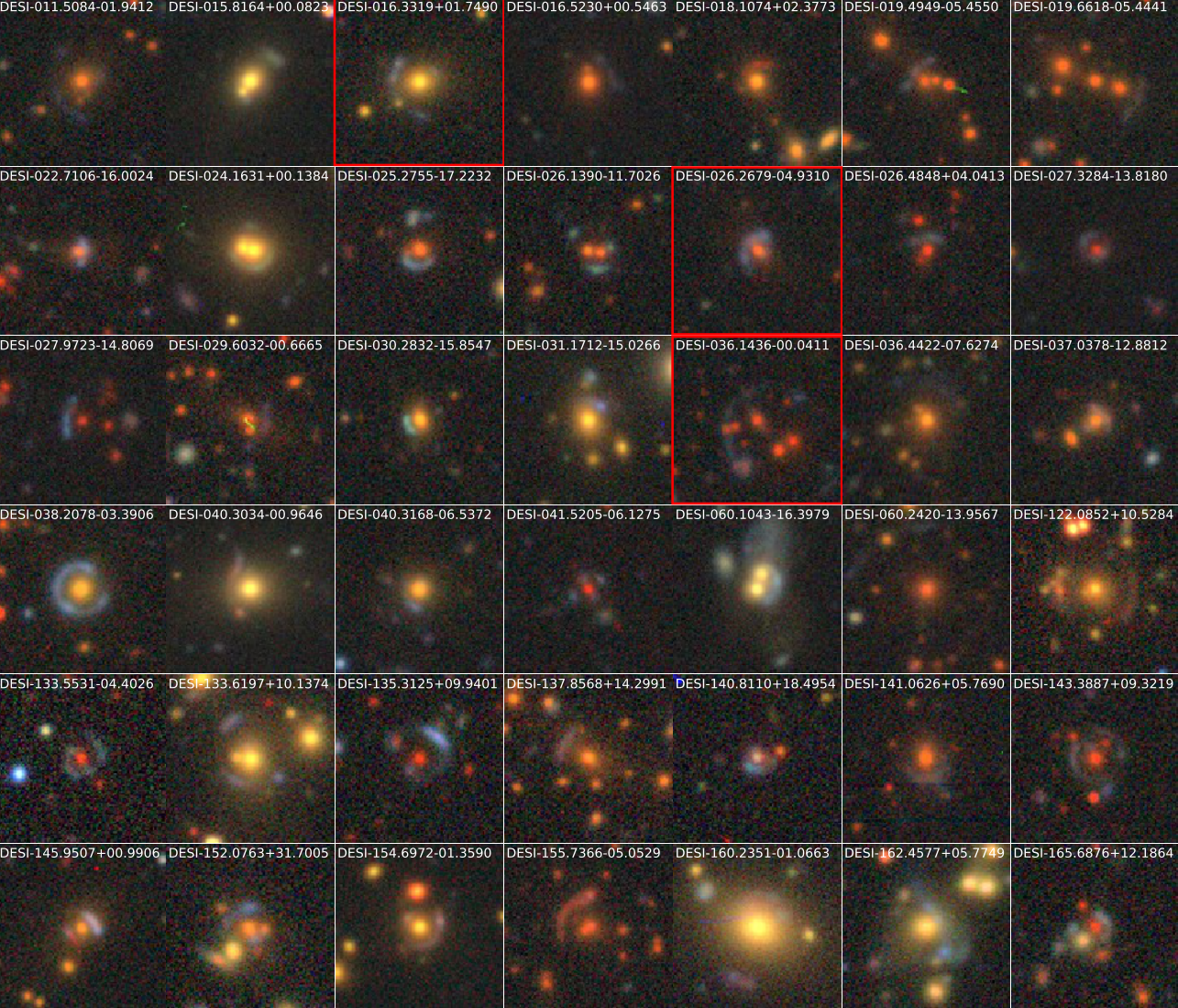
CMU DeepLens in the wild
Huang et al. (2019) - arXiv:1906.00970
takeaway message
Deep Learning for Low Level Processing
- An example of Deep Learning allowing us to handle the volume and data rate at the image level
- Our automated lens finder is faster and more reliable than human volunteers.
$\Longrightarrow$ Larger and more robust samples for the science analysis.
Hybrid physics-ML models for image inverse problems
Work in collaboration with:
Peter Melchior, Fred Moolekamp
$\Longrightarrow$ Use PixelCNNs as deep priors for deblending
The challenge of galaxy blending


Bosch et al. 2017
- In HSC over 60% of all galaxies are blended
- Important impact on our main cosmological probes
- Current generation of deblenders does not meet our target requirements
- Existing methods rely on simple assumptions about galaxy profiles, like symmetry or monotonicity
Deblending is an ill-posed inverse problem, akin to Blind Source Separation. The is no single solution.
$\Longrightarrow$ Intuitively, the key will to leverage an understanding of how individual galaxies look like.
$\Longrightarrow$ Intuitively, the key will to leverage an understanding of how individual galaxies look like.
Can AI solve all of our problems?
Branched GAN model for deblending (Reiman & Göhre, 2018)

The issue with using deep learning as a black-box
- No explicit control of noise, PSF, depth, number of sources.
- Model would have to be retrained for all observing configurations
- No guarantees on the network output (e.g. flux preservation, artifacts)
- No proper uncertainty quantification.

Linear inverse problems
$\boxed{y = \mathbf{A}x + n}$$\mathbf{A}$ is known and encodes our physical understanding of the problem.
$\Longrightarrow$ When non-invertible or ill-conditioned, the inverse problem is ill-posed with no unique solution $x$
 Deconvolution
 Inpainting
 Denoising
The Bayesian view of the problem:
$$ p(x | y) \propto p(y | x) \ p(x) $$
- $p(y | x)$ is the data likelihood, which contains the physics
- $p(x)$ is our prior knowledge on the solution.
With these concepts in hand, we want to estimate the Maximum A Posteriori solution:
$$\hat{x} = \arg\max\limits_x \ \log p(y \ | \ x) + \log p(x)$$
For instance, if $n$ is Gaussian, $\hat{x} = \arg\max\limits_x \ \frac{1}{2} \parallel y - \mathbf{A} x \parallel_{\mathbf{\Sigma}}^2 + \log p(x)$
$$\hat{x} = \arg\max\limits_x \ \log p(y \ | \ x) + \log p(x)$$
For instance, if $n$ is Gaussian, $\hat{x} = \arg\max\limits_x \ \frac{1}{2} \parallel y - \mathbf{A} x \parallel_{\mathbf{\Sigma}}^2 + \log p(x)$
How do you choose the prior ?
Classical examples of signal priors
Sparse
![]()
$$ \log p(x) = \parallel \mathbf{W} x \parallel_1 $$

$$ \log p(x) = \parallel \mathbf{W} x \parallel_1 $$
Gaussian
![]() $$ \log p(x) = x^t \mathbf{\Sigma^{-1}} x $$
$$ \log p(x) = x^t \mathbf{\Sigma^{-1}} x $$
 $$ \log p(x) = x^t \mathbf{\Sigma^{-1}} x $$
Total Variation
![]() $$ \log p(x) = \parallel \nabla x \parallel_1 $$
$$ \log p(x) = \parallel \nabla x \parallel_1 $$
But what about this?
Can we use Deep Learning to learn the prior from data?
The evolution of generative models


- Deep Belief Network
(Hinton et al. 2006) - Variational AutoEncoder
(Kingma & Welling 2014) - Generative Adversarial Network
(Goodfellow et al. 2014) - Wasserstein GAN
(Arjovsky et al. 2017)
A visual Turing test
Fake PixelCNN samples

Real SDSS
Not all generative models are created equal

Grathwohl et al. 2018
- GANs and VAEs are very common and successfull but do not fit our purposes.
- We want a model which can provide an explicit $\log p(x)$.
PixelCNN: Likelihood-based Autoregressive generative model
Models the probability $p(x)$ of an image $x$ as:
$$ p_{\theta}(x) = \prod_{i=0}^{n} p_{\theta}(x_i | x_{i-1} \ldots x_0) $$
![]()
- Some of the best log-likelihoods on the market.
- Extremely stable during training.
- Slow to sample from.

Ramachandran et al. 2017
van den Oord et al. 2016
- Provides an explicit value for $\log p_\theta(x)$
$\Longrightarrow$ Can be used as a Bayesian prior for inverse problems.
A deep denoising example
$$ \boxed{{\color{Orchid} y} = {\color{SkyBlue} x} + n} $$
Try me out at: https://eiffl.github.io/DeepPriors
- We learn the distribution of noiseless data $\log p_\theta(x)$ from samples using a deep generative model.
- We measure a noisy ${\color{Orchid} y}$ and we want to estimate a denoised ${\color{SkyBlue} x}$
- The solution should lie on the realistic data manifold, symbolized by the two-moons distribution.
We want to solve for the Maximum A Posterior solution:
$$\arg \max - \frac{1}{2} \parallel {\color{Orchid} y} - {\color{SkyBlue} x} \parallel_2^2 + \log p_\theta({\color{SkyBlue} x})$$ This can be done by gradient descent as long as one has access to $\frac{\color{orange} d \color{orange}\log \color{orange}p\color{orange}(\color{orange}x\color{orange})}{\color{orange} d \color{orange}x}$.
The Scarlet algorithm: deblending as an optimization problem
Melchior et al. 2018
$$ \mathcal{L} = \frac{1}{2} \parallel \mathbf{\Sigma}^{-1/2} (\ Y - P \ast A S \ ) \parallel_2^2 - \sum_{i=1}^K \log p_{\theta}(S_i) + \sum_{i=1}^K g_i(A_i) + \sum_{i=1}^K f_i(S_i)$$
Where for a $K$ component blend:
- $P$ is the convolution with the instrumental response
- $A_i$ are channel-wise galaxy SEDs, $S_i$ are the morphology models
- $\mathbf{\Sigma}$ is the noise covariance
- $\log p_\theta$ is a PixelCNN prior
- $f_i$ and $g_i$ are arbitrary additional non-smooth consraints, e.g. positivity, monotonicity...
Training the morphology prior

Postage stamps of isolated COSMOS galaxies used for training, at WFIRST resolution and fixed fiducial PSF
isolated galaxy
![]() $\log p_\theta(x) = 3293.7$
$\log p_\theta(x) = 3293.7$
 $\log p_\theta(x) = 3293.7$
artificial blend
![]() $\log p_\theta(x) = 3100.5 $
$\log p_\theta(x) = 3100.5 $
 $\log p_\theta(x) = 3100.5 $
Scarlet in action
Input blend
![]()

Solution
![]()
![]()


Residuals
![]()
![]()


- Classic priors (monotonicity, symmetry).
- Deep Morphology prior.
True Galaxy
![]()

Deep Morphology Prior Solution
![]()

Monotonicity + Symmetry Solution
![]()

Extending to multi-band images

Lanusse, Melchior, Moolekamp (2019)
Takeaway
- Deep generative models can be used to provide data driven priors.
- Explicit likelihood, uses of all of our physical knowledge.
$\Longrightarrow$ The method can be applied for varying PSF, noise, or even different instruments! - Iterative optimization can include additional regularization terms.
- Ensures fit to data (flux preservation).
- Can impose physical constraints like positivity.
But what about uncertainty quantification?
Can we sample from the full Bayesian posterior $p(y | x)$ to estimate uncertainties?
Deep Posterior Sampling with Denoising Score Matching
Work in collaboration with:
Benjamin Remy, Zaccharie Ramzi
$\Longrightarrow$ Sample from posterior with gradient-based Monte-Carlo methods

The score is all you need!
- Instead of learning ${\color{orange} \log {\color{orange} p\color{orange}(\color{orange} x\color{orange})}}$, learn $\frac{\color{orange} d \color{orange}\log \color{orange}p\color{orange}(\color{orange}x\color{orange})}{\color{orange} d
\color{orange}x}$, a.k.a. the Score Function
- MAP estimation only need the score! Same is true for Hamiltonian Monte Carlo!
- The score can be learned efficiently by training a deep Gaussian denoiser (Denoising Score Matching).
- The score of the full posterior is simply: $$\nabla \log p(x |y) = \underbrace{\nabla \log p(y |x)}_{\mbox{known}} \quad + \quad \underbrace{\nabla \log p(x)}_{\mbox{learned}}$$

$\boldsymbol{x}'$
$\boldsymbol{x}$
$\boldsymbol{x}'- \boldsymbol{r}^\star(\boldsymbol{x}', \sigma)$
$\boldsymbol{r}^\star(\boldsymbol{x}', \sigma)$
 $$\boxed{\boldsymbol{r}^\star(\boldsymbol{x}', \sigma) = \boldsymbol{x}' + \sigma^2 \nabla_{\boldsymbol{x}} \log p_{\sigma^2}(\boldsymbol{x}')}$$
Uncertainty quantification in Magnetic Resonance Imaging (MRI)
Ramzi, Remy, Lanusse et al. 2020 
$$\boxed{y = \mathbf{M} \mathbf{F} x + n}$$
- Learn score $\nabla \log p(x)$ with UNet trained by denoising score matching.
- Sample 320x320pix image posterior by Annealed Hamiltonian Monte Carlo.
$\Longrightarrow$ We can see which parts of the image are well constrained by data, and which regions are uncertain.
Probabilistic Mass-Mapping of the HST COSMOS field
Remy, Lanusse, Ramzi et al. 2020 
$$\boxed{\gamma = \mathbf{P} \kappa + n}$$

- Hybrid prior: theoretical Gaussian on large scale, data-driven on small scales using N-body simulations. $$\underbrace{\nabla_{\boldsymbol{\kappa}} \log p(\boldsymbol{\kappa})}_\text{full prior} = \underbrace{\nabla_{\boldsymbol{\kappa}} \log p_{th}(\boldsymbol{\kappa})}_\text{gaussian prior} + \underbrace{\boldsymbol{r}_\theta(\boldsymbol{\kappa}, \nabla_{\boldsymbol{\kappa}} \log p_{th}(\boldsymbol{\kappa}))}_\text{learned residuals}$$ with $p_{th}(\boldsymbol{\kappa}) = \frac{1}{ \sqrt{ \det 2 \pi \boldsymbol{S}}} \exp \left( -\frac{1}{2} \boldsymbol{\kappa}^\dagger \boldsymbol{S}^{-1} \boldsymbol{\kappa} \right)$, computed from theory.
Conclusion
Where is Deep Learning interesting for Astronomical Image Processing?
- Extremely efficient at classification tasks.
$\Longrightarrow$ Improve size and quality of samples for science. - Restricting Deep Learning to modeling the priors brings robustness and intrepretability.
- Deep Generative Models are perfect for learning data-driven priors.
- Proper Uncertainty Quantification is possible by sampling the Bayesian posterior of the inverse problem.
Thank you!
Bonus: How to train a generative model from noisy/corrupted data?
Deep Generative Models for Galaxy Image Simulations
Work in collaboration with
Rachel Mandelbaum, Siamak Ravanbakhsh, Chun-Liang Li, Barnabas Poczos, Peter Freeman
Lanusse et al. (2020)
Ravanbakhsh, Lanusse, et al. (2017)
Ravanbakhsh, Lanusse, et al. (2017)
The weak lensing shape measurement problem

Shape measurement biases
$$ < e > = \ (1 + m) \ \gamma \ + \ c $$
- Can be calibrated on image simulations
- How complex do the simulations need to be?
Complications specific to astronomical images: spot the differences!

CelebA

HSC PDR-2 wide
- There is noise
- We have a Point Spread Function
A Physicist's approach: let's build a model


$\longrightarrow$
$g_\theta$
$g_\theta$
$\longrightarrow$
PSF
PSF
$\longrightarrow$
Pixelation
Pixelation
$\longrightarrow$
Noise
Noise


Probabilistic model
$$ x \sim ? $$
$$ x \sim \mathcal{N}(z, \Sigma) \quad z \sim ? $$
latent $z$ is a denoised galaxy image
latent $z$ is a denoised galaxy image
$$ x \sim \mathcal{N}( \mathbf{P} z, \Sigma) \quad z \sim ?$$
latent $z$ is a super-resolved and denoised galaxy image
latent $z$ is a super-resolved and denoised galaxy image
$$ x \sim \mathcal{N}( \mathbf{P} (\Pi \ast z), \Sigma) \quad z \sim ? $$
latent $z$ is a deconvolved, super-resolved, and denoised galaxy image
latent $z$ is a deconvolved, super-resolved, and denoised galaxy image
$$ x \sim \mathcal{N}( \mathbf{P} (\Pi \ast g_\theta(z)), \Sigma) \quad z \sim \mathcal{N}(0, \mathbf{I}) $$
latent $z$ is a Gaussian sample
$\theta$ are parameters of the model
latent $z$ is a Gaussian sample
$\theta$ are parameters of the model
$\Longrightarrow$ Decouples the morphology model from the observing conditions.
How to train your dragon model

- Training the generative amounts to finding $\theta_\star$ that
maximizes the marginal likelihood of the model:
$$p_\theta(x | \Sigma, \Pi) = \int \mathcal{N}( \Pi \ast g_\theta(z), \Sigma) \ p(z) \ dz$$
$\Longrightarrow$ This is generally intractable
- Efficient training of parameter $\theta$ is made possible by Amortized Variational Inference.
Auto-Encoding Variational Bayes (Kingma & Welling, 2014)
- We introduce a parametric distribution $q_\phi(z | x, \Pi, \Sigma)$ which aims to model the posterior $p_{\theta}(z | x, \Pi, \Sigma)$.
- Working out the KL divergence between these two distributions leads to: $$\log p_\theta(x | \Sigma, \Pi) \quad \geq \quad - \mathbb{D}_{KL}\left( q_\phi(z | x, \Sigma, \Pi) \parallel p(z) \right) \quad + \quad \mathbb{E}_{z \sim q_{\phi}(. | x, \Sigma, \Pi)} \left[ \log p_\theta(x | z, \Sigma, \Pi) \right]$$ $\Longrightarrow$ This is the Evidence Lower-Bound, which is differentiable with respect to $\theta$ and $\phi$.
The famous Variational Auto-Encoder

$$\log p_\theta(x| \Sigma, \Pi ) \geq - \underbrace{\mathbb{D}_{KL}\left( q_\phi(z | x, \Sigma, \Pi) \parallel p(z) \right)}_{\mbox{code regularization}} + \underbrace{\mathbb{E}_{z \sim q_{\phi}(. | x, \Sigma, \Pi)} \left[ \log p_\theta(x | z, \Sigma, \Pi) \right]}_{\mbox{reconstruction error}} $$
Sampling from the model
 Woups... what's going on?

Tradeoff between code regularization and image quality
$$\log p_\theta(x| \Sigma, \Pi ) \geq - \underbrace{\mathbb{D}_{KL}\left( q_\phi(z | x, \Sigma, \Pi) \parallel p(z) \right)}_{\mbox{code regularization}} + \underbrace{\mathbb{E}_{z \sim q_{\phi}(. | x, \Sigma, \Pi)} \left[ \log p_\theta(x | z, \Sigma, \Pi) \right]}_{\mbox{reconstruction error}} $$

Latent space modeling with Normalizing Flows
$\Longrightarrow$ All we need to do is sample from the aggregate posterior of the data instead of sampling from the prior.


Dinh et al. 2016
Normalizing Flows
- Assumes a bijective mapping between data space $x$ and latent space $z$ with prior $p(z)$: $$ z = f_{\theta} ( x ) \qquad \mbox{and} \qquad x = f^{-1}_{\theta}(z)$$
- Admits an explicit marginal likelihood: $$ \log p_\theta(x) = \log p(z) + \log \left| \frac{\partial f_\theta}{\partial x} \right|(x) $$
Flow-VAE samples

Second order moments


Testing galaxy morphologies

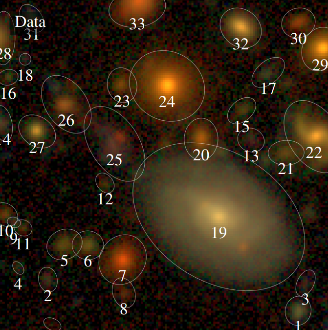
Bayesian Inference a.k.a. Uncertainty Quantification
The Bayesian view of the problem:
$$ p(z | x ) \propto p_\theta(x | z, \Sigma, \mathbf{\Pi}) p(z)$$
where:
- $p( z | x )$ is the posterior
- $p( x | z )$ is the data likelihood, contains the physics
- $p( z )$ is the prior
Data
$x_n$
$x_n$
Truth
$x_0$
$x_0$
Posterior samples
$g_\theta(z)$
$g_\theta(z)$

$\mathbf{P} (\Pi \ast g_\theta(z))$
Median

Data residuals
$x_n - \mathbf{P} (\Pi \ast g_\theta(z))$
$x_n - \mathbf{P} (\Pi \ast g_\theta(z))$
Standard Deviation
$\Longrightarrow$ Uncertainties are fully captured by the posterior.
How to perform efficient posterior inference?


- Posterior fitting by Variational Inference
$$ \mathrm{ELBO} = - \mathbb{D}_{KL}\left( q_\phi(z) \parallel p(z) \right) \quad + \quad \mathbb{E}_{z \sim q_{\phi}} \left[ \log p_\theta(x_n | z, \Sigma_n, \Pi_n) \right]$$ - Posterior fitting by $EL_{2}O$
$$EL_2O = \arg \min_\theta \mathbb{E}_{z \sim p^{\prime}} \sum_i \alpha_i \parallel \nabla_{z}^n \ln q_\theta(z) - \nabla_{z}^{n} \ln p(z | x_n, \Sigma_n, \Pi_n) \parallel_2^2$$See (Seljak & Yu, 2019) for more details. - Or your favorite method...